Task Description

The objective of our work was to develop a classifier of different types of stellar objects. The information available about those objects was the radius, the position in the sky in celestial coordinates, and the time series of 16 points (4 each night, 4 nights). We decided to use a decision tree for this purpose, in order to classify from general objects like galaxies or stars to specific subclasses of variable stars. The decisions include probabilities, so at the end we have a probability of belonging at each terminal class.

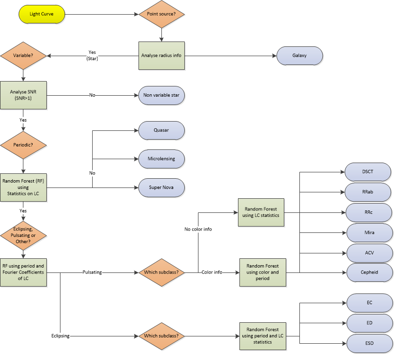
Star/galaxy clasifier

The information used for this classifier is only the radius information. Stars should be point sources, with a radius of less than a certain number of pixels and without big variations from one epoch to another.

Variability test

We found that the derived photometric error of our data tend to be too small, which made most of our sources look like variable, while realistically less than 10% of the stellar objects are variable. We thus first correct the error bars using the method introduced by Protopapas et al. (2013). The idea is that for a non-variable source, the error bar should be comparable to the interquartile range of the source magnitude. For Ns sources in a given CCD we fit an error correction parameter which minimizes

\alpha_{cf}=arg min_{\alpha}\sum_{k=1}^{N_s}\left(iqr({y}_k)-\alpha\cdot med({e}_k)\right)^2

Where y_k and e_k are the magnitudes and error bars of the lightcurve of source k, respectively, iqr is the interquartile range and med is the median.

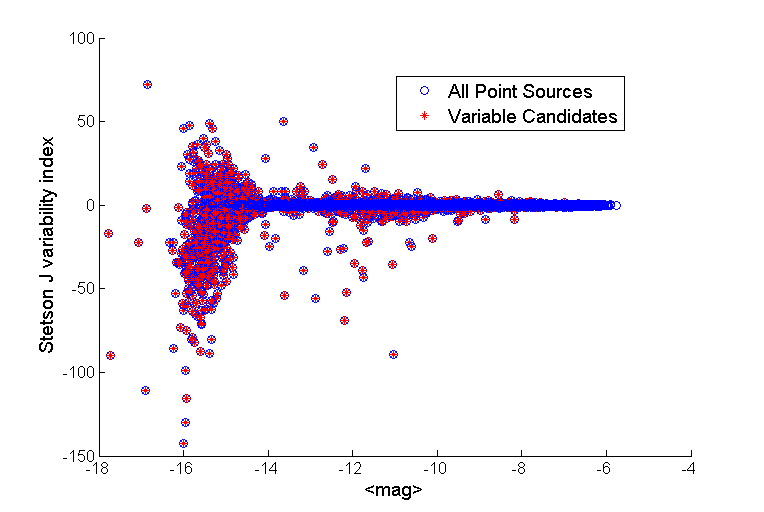
After the correction, we use the Stetson J index (Stetson 1996) to test the variability of the source. It is a robust method to decide if a time series shows variability or not, relating the measurements and the error associated with those. The equations for that index are the following:

J=\frac{\sum_{k=1}^n w_k\cdot sgn(P_k)\cdot\sqrt{\abs{P_k}}}{\sum_{k=1}^nw_k}

P_k=\delta_{i(k)}\delta_{j(k)}\delta=\sqrt{\frac{n}{n-1}}\frac{y-\bar{y}}{e}

We use |J| >1 as a criteria for choosing variable candidates. In this step, 1780 out of 68739 point sources were labeled as variable candidates. Figure below highlights the variable candidates with red cross among all of our point sources shown with blue circles. In the figure is possible to see that objects with a Stetson J index close to zero are most likely non-variable object, while if the absolute value of the index is greater than zero, that object should be a variable one.

Periodic discrimination

One subclass of variable objects that are important to separate are the periodic ones. Although there are other variable stellar objects that also could be interesting to identify. With that idea, we developed a classifier that can associate probabilities of belong to every of the following classes:

Periodic: encompasses objects that vary cyclically with time. Within this group are included, for example, pulsating stars and eclipsing systems and subclassifications. As they vary with a period is possible to observe these variables in multiple cycles to more accurately determine its parameters, e.g. size, distance, temperature and even separation between binary stars.

Quasar:: or quasi-stellar radio source is an AGN (active galactic nucleus) that is very distant from us but extremely energetic. Consist of a supermassive black hole that interacts irregularly with the material of the host galaxy, this is why we see random variations in their behavior.

Microlensing: astrophysical effect that greatly increase the brightness of a distant object through another closer aligned, serving as 'magnifying glass'. The intermediate object can be a star, planet or moon while there is an alignment with the background source.

Supernova: is a stellar explosion as the last step of the evolution of a star. They are extremely bright, sometimes more than an entire galaxy, and its brightness will drastically increase in the first days and then decline over several weeks or months due to radioactive material is expelled. This event is the primarily responsible for the chemical enrichment of the universe, all elements heavier than iron are produced in this explosion.

The light curve information was obtained from several databases including:
OGLE (Optical Gravitational Lensing Experiment): periodic and microlensing database.
MACHO (MAssive Compact Halo Objects): quasar database.
CfA (Center for Astrophysics): SNe database.

This classifier is a random forest trained with statistical values obtained from the light curves of each object. Those statistics are the following:

Statistic	Description
Standard Deviation	This statistic shows how much variation or dispersion from the average exists
Skewness	Statistic that measures the asymmetry of the distribution of the samples. In this cases, we compute the skewness of the flux measurements for each lightcurve.
Kurtosis	Another statistic related to the shape of the data. Kurtosis measures the peaks of the data, and how far away are from the mean.
Median Absolute Deviation	Measure related to the distance between the samples and the median value of them. It is robust when only few data points are available.
Interquartile Range	Measure of the dispersion of the distribution. It’s compute as the first quartile (we there is the higher 25% of the data) minus the third quartile (with the lower 25% of the data).
Stetson J index	Variability index
QSO index	Variability index for quasar identification. Proposed by Butler and Bloom on 2011.
Non-QSO index	Fit statistic for non-QSO variable star.

Type of periodic star

After we decide that there is a chance that one source is periodic, we perform a classification between two kinds of periodic stars: Eclipsing and Pulsating. This is a rough classification, and in each class we can find several different subclasses, that are going to be used in forward decisions.

Once again, the Machine Learning algorithm used is Random Forest. This time the features used are related to the period and the shape of the lightcurves. We only use two features in this classifier: period, found by Lomb Scargle, and Fourier coefficient A_{21}. This coefficient is calculated as the ratio between the amplitudes of the second and first harmonic wave fitted to the light-curve.

This classifier performs almost perfectly on the training set, but in the real data that doesn’t happen. That is because the Fourier coefficient depends on the used period, so if the period is miscalculated, then the estimation of the coefficient is not going to be accurate. Nevertheless, if the amount of information increases, then the classification should be more robust.

Subtype of Pulsating star

In this stage we perform two different classifiers. That is because we look for the color information on the USNO-B1.0 (B and R) and 2MASS (J, H and Ks) catalog, but is not available for each stellar object that we have. The color information is useful to separate different classes of pulsating stars with more confidence. When we don’t have color information, we run a Random Forest classifier with the same statistical information than in the Periodic discrimination.

The different kinds of pulsating stars that we want to discriminate are:

DSCT: stars that are on the main sequence (like the Sun that burns hydrogen at its core) and having its surface pulsations are of this kind. Its pulse period goes between 0.03 to 0.3 days and have a maximum amplitude of 0.9 magnitudes in optical wavelengths. His color is blue because its surface temperature fluctuates depending on the star between 7500 and 10000 K.

RRab: belong to this group are the stars on the Horizontal Branch (helium burning phase in its core) and pulsating periodically between 0.3 up to 1.2 days. Their amplitudes are high, 0.5 to 2 magnitudes, so they are constantly used as standard candles to measuring distances in galactic and extragalactic scales.

RRc: are the same type as RRab, but their periods are ranging from 0.2 to 0.4 days. Their amplitudes are also lower, reaching only 0.8 magnitudes due to they are pulsating in the first overtone.

Mira: giant stars are long-period (80-1000 days) that are in the phase of AGB (Asymptotic Giant Branch), which is the last step before they die and become a white dwarf. Because of its size the amplitudes are huge (from 2.5 to 11 magnitudes) and red colors predominate because of its low surface temperature (about 3000 K).

ACV: this variable has very marked rotation and magnetic fields that vary on a time scale of 0.5 to 160 days. Brightness changes in this time period between 0.01 and 0.1 magnitudes in V. It is characterized by rare chemical elements and high surface temperatures (10000-25000 K) so their colors are bluer.

Cepheid: pulsating stars with high surface brightness and cycles from 1 to 135 days. Its ranges from tenths to 2 magnitudes. Follow a relationship that binds their period and luminosity, so that together with its amplitude are useful for measuring galactic and extragalactic distance scales. Its temperature ranges from 5500 K, with redness in the minimum brightness and 7500 K, bluish at maximum brightness.

Subtype of Eclipsing Star

For eclipsing variable stars, the color information is not useful, because this type is extrinsic. This means that the variability is not associated with the physical properties of the star. For this reason, this kind of stars may be on any color and in a broad range of periods. The classifier is trained again with statistical information and the fourier coefficients A21 and A31.

The subtypes of eclipsing stars that we want to classify are:

EC: contact binaries with periods usually shorter than 1 day. Can not be distinguished between the two components so it is impossible to know the beginning and end of the eclipses. Their amplitudes are less than 0.8 mag. in optical bands and surface temperature about 6000 K (reddish color).

ED: detached eclipsing binaries for which it is possible to distinguish a plateau between eclipses. It is common to see an asymmetry between the size of the eclipses, but is only related to the size and color of the secondary star. Their periods and amplitudes varies in all ranges as it depends on the configuration of the binary system.

ESD: semi-detached eclipsing binaries. For this type one can not differentiate between eclipses because their continuous succession. Generally have periods of 1 day and blue colors related to 10000-30000 K for the surface temperature.