Introduction

The Victor M. Blanco telescope at the observatory cerro tololo (CTIO) is one of the telescopes used in the 90’s decade to measure the expansion of the universe and its deceleration, but the astronomers got surprised when they discovered that indeed it was being the opposite, the expansion was being accelerated by something. A new instrument called the Dark Energy Camera (DECam) was installed in 2012.

This camera contains 61 CCD’s, each one of 520 Mpix and a total field of view of 2.2 degrees. It was designed to make surveys of extragalactic objects to have a better comprehension of what is causing this accelerated expansion.

The Chile-Harvard Innovative Learning Exchange Program, in which students from various background worked on such data sets in Chile for two weeks.

Data

• Raw CCD images from the Victor M. Blanco Telescope’s Dark Energy Camera (DECam) at CTIO.
• 64 CCDs / 40 fields of view / 16 epochs over 4 nights.
• Over 1 TB of raw image data per night.
• Unique combination of cadence, depth and field of view.
• Allows the study of objects that vary in the U band with time-scales of a few hours in a large volume of the Universe.

Aim

Develop fast, cost-effective computational methods to process and analyze DECam data in order to construct light curves in the U band.

Procedure

1. Detect pixels with high values and measure the background level and noise:

For each CCD, we first identify the pixels with large ADU values using 99.6% quantile This gives a binary image of 'bright pixels', which are possible sources, and 'faint pixels', which we use to estimate background.

2. Identify blocks:

We single out possible sources by finding the smallest blocks containing connected 'bright pixels'.

3. Cosmic rays test:

For each small block, we calculate the skewness and kurtosis of the observed ADUs to rule out cosmic rays.

4. Gaussian fit: position, shape, pixel coordinates:

We fit a Gaussian model to construct a catalogue containing positions (\mu_{x}, \ \mu_{y}) , flux A , spread (\sigma_{x}, \ \sigma_{y}) , inclination \rho and errors of the the sources for each CCD, field and epoch.

I_{x,y}= \frac{A}{2 \pi \sigma_{x} \sigma_{y}\sqrt{1-\rho^{2}}}exp(-\frac{1}{1-\rho^{2}}[\frac{(x-\mu_{x})^{2}}{2\sigma_{x}^{2}}+\frac{(y-\mu_{y})^{2}}{2\sigma_{y}^{2}}-\frac{\rho (x-\mu_{x})(y-\mu_{y})}{\sigma_{x} \sigma_{y}}])

In the following image is presented a 1D cut of the CCD centered on a star and the corresponding gaussian fit.



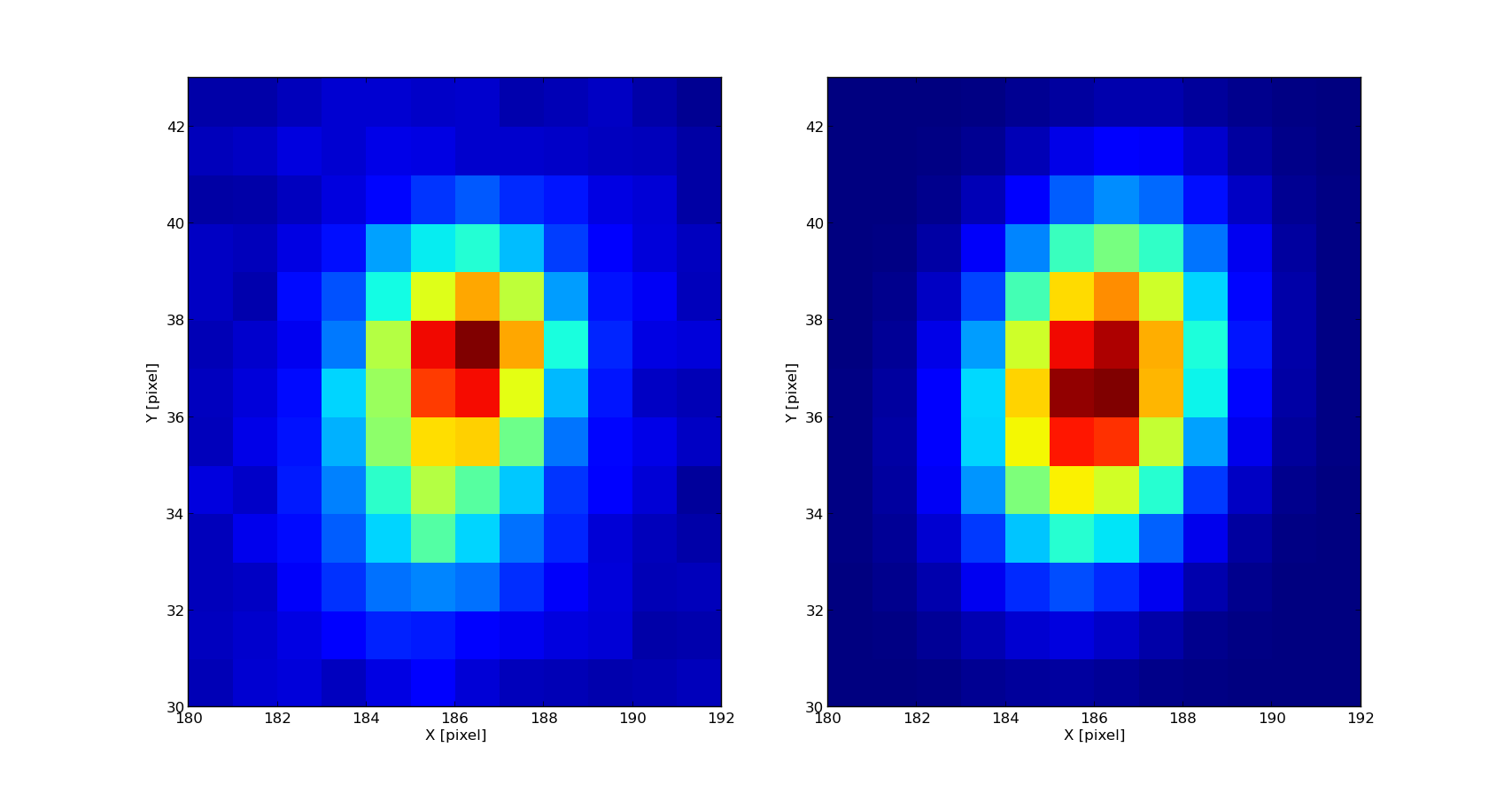
A heat map comparing the raw image and the model image after the gaussian fit is presented below.



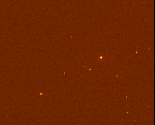
An example of just a fraction of a CCD image with stars and cosmic rays.



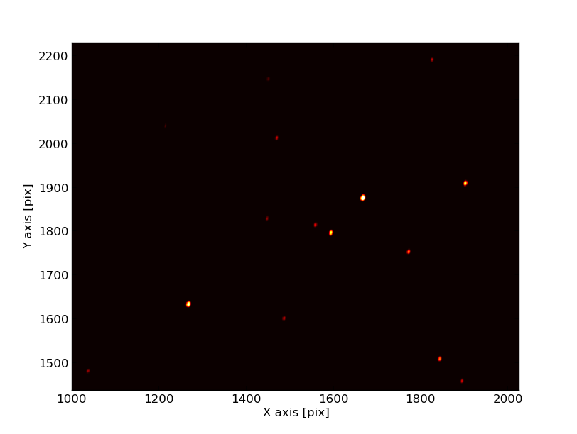
And its corresponding model image after we found the sources and performed the fit.


5. Transform to celestial world coordinates:

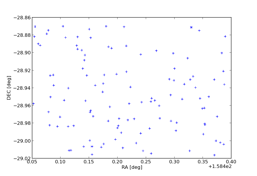
Using the header information of each fits file, we transform the position of the sources and its errors to world celestial coordinates (Right Ascension and Declination). An example of a arbitrary region of one of the 40 fields is presented below.


6. Calibration with Standard stars from the Sloan Digital Sky Survey (SDSS):

The previous steps were done also for observations pointing to standard fields. One of them was a field covered by the Sloan Digital Sky Survey, and it was used for transform from ADU to magnitudes in the U band.

7. Matching between epochs:

Finally we took the 16 corresponding catalogues for each CCD and field. Using the position in celestial coordinates and its errors in each epoch, we performed a matching of the objects through the different epochs. After this we had 16 catalogues for the same region of the sky, with a ID for each object and its magnitudes at different epochs, i.e. we obtaied light curves for the different objects found in the 40 fields.

Future work

• Improve the cosmic ray detection.
• Add gaussian mixture in order to detext sources that could be very close.
• Use a more realistic profile for the Point Spread Function (PSF)
• Use others standard fields.
• Improve the distance function using additional measurement like the flux (or something similar) in the object-matching process.